Approach
Geophysical Inversion
The strong response of brightness temperature to change in soil moisture forms the basis of passive microwave remote sensing of soil moisture. This relationship between brightness temperature and soil moisture can be modeled as a zeroth order radiative transfer process known as the τ-ω ("tau-omega") model. This model is so named because it incorporates the impacts of attenuation (τ) and scattering (ω) of aboveground vegetation into the overall microwave emission by the combined soil-vegetation medium. There is a long heritage in successful deployment of this model for soil moisture estimation using brightness temperature observations acquired on vehicle-mounted, airborne, and spaceborne radiometers. The majority of satellite-based soil moisture estimates to date are based on geophysical inversion of this simple but effective model. There is an abundant amount of review literature devoted to the use of this model in soil moisture estimation at various spatial scales. Here we will list one that provides a succinct and comprehensive description of the model.
Njoku, E and Li, L. 1999. "Retrieval of Land Surface Parameters Using Passive Microwave Measurements at 6-18 GHz," IEEE Trans. Geosci. and Remote Sens, 37(1), p. 79-93.
In its analytical form, the τ-ω model relates brightness temperature to soil moisture with correction in surface temperature, soil attributes, and the impacts of vegetation attenuation, emission, and scattering.
TB = Teff [ ( 1 − rs ) e-τ + ( 1 − ω ) ( 1 − e-τ ) ( 1 + rs e-τ ) ]
where Teff is the effective soil temperature in Kelvins, rs is the Fresnel reflectivity after rough surface modulation, τ is the vegetation opacity given by τ = b VWC / cos(θ) [note: VWC = vegetation water content in kg/m2 and θ is the angle at which TB is observed], and ω is the single-scattering albedo of vegetation. Parameters that are in boldface assumed to exhibit polarization dependence. In reality, however, τ and ω will likely have polarization dependence as well.
The Single Channel Algorithm (SCA) was used in this investigation due its simplicity and effectiveness. Our SCA implementation follows a simple linear interpolation approach, in that a vector that spans between the low and high ends of physically possible soil moisture values goes into a soil dielectric model. The resulting complex dielectric constants are then used to derive the Fresnel reflectivities, followed by Teff correction, roughness correction, as well as correction for vegetation attenuation, emission, and scattering to produce the forward-modeled brightness temperature values. Because this brightness temperature vector has a one-to-one correspondence with the underlying soil moisture vector, one can obtain the corresponding satellite-based soil moisture estimate by simple linear interpolation. This is also the same operational implementation of SCA in SMAP.
Implicit in this τ-ω forward model is its parameterization based on land cover types. To this end, we use the same MODIS/Terra+Aqua Land Cover Type Yearly L3 Global 500 m SIN Grid (MCD12Q1) Data Product deployed in SMAP operational code. In essence, unique values of τ, ω, and surface roughness correction are assigned on a per-pixel basis based on the IGBP land cover classification scheme provided in MCD12Q1. Below is the lookup table that maps individual IGBP land cover types to their corresponding τ-ω parameters:
| ID | MODIS IGBP Land Classification | h | b | ω | stem factor |
|---|---|---|---|---|---|
| 0 | Water | 0.000 | 0.000 | 0.000 | -- |
| 1 | Evergreen Needleleaf Forests | 0.160 | 0.100 | 0.070 | 15.960 |
| 2 | Evergreen Broadleaf Forests | 0.160 | 0.100 | 0.070 | 19.150 |
| 3 | Deciduous Needleleaf Forests | 0.160 | 0.120 | 0.070 | 7.980 |
| 4 | Deciduous Broadleaf Forests | 0.160 | 0.120 | 0.070 | 12.770 |
| 5 | Mixed Forests | 0.160 | 0.110 | 0.070 | 12.770 |
| 6 | Closed Shrublands | 0.110 | 0.110 | 0.050 | 3.000 |
| 7 | Open Shrublands | 0.110 | 0.110 | 0.050 | 1.500 |
| 8 | Woody Savannas | 0.125 | 0.110 | 0.050 | 4.000 |
| 9 | Savannas | 0.156 | 0.110 | 0.080 | 3.000 |
| 10 | Grasslands | 0.156 | 0.130 | 0.050 | 1.500 |
| 11 | Permanent Wetlands | 0.000 | 0.000 | 0.000 | 4.000 |
| 12 | Croplands | 0.108 | 0.110 | 0.050 | 3.500 |
| 13 | Urban and Built-up Lands | 0.000 | 0.100 | 0.030 | 6.490 |
| 14 | Cropland/Natural Vegetation Mosaics | 0.130 | 0.110 | 0.065 | 3.250 |
| 15 | Snow and Ice | 0.000 | 0.000 | 0.000 | 0.000 |
| 16 | Barren | 0.150 | 0.000 | 0.000 | 0.000 |
The same table can also be found in the SMAP Algorithm Theoretical Basis Document: Level 2 and 3 Soil Moisture (Passive) Products document.
Intercalibration
This investigation has a single focus on the development of a long-term consistent soil moisture data record. Here, consistency means consistency in the calibration of the original satellite observations that are used to derive soil moisture estimates. The two groups of satellites that comprise the X- and L-band brightness temperature observations follow two distinct intercalibration schemes detailed as follows.
L-band (1.4 GHz; λ ~ 20 cm)
Both SMOS and SMAP acquire brightness temperature observations at L-band frequencies at about the same 36-km spatial resolution and at about the same 2-3 day average global revisit period. SMAP observes brightness temperatures at a fixed incidence angle of 40º, whereas SMOS, by virtue of its interferometric approach, observes brightness temperatures at multiple incidence angles all at the same time. To achieve a long-term consistent brightness temperature data record, SMOS' brightness temperatures at 40º were extracted and combined with SMAP's brightness temperatures at 40º to produce a contiguous record starting from about 2010 to present. Since only two L-band observing platforms are involved in this combined record, calibration consistency can be accomplished by relative calibration. In this investigation, SMAP brightness temperatures were used as the calibration reference for SMOS' brightness temperatures.
To this end, matchup pairs between SMAP and SMOS observations were first extracted. These matchup pairs were subject to these stringent space-time colocation criteria:
- Boresights fall within a 1-km grid cell
- Azimuth angles within ±2.5º
- Observation times within ±2.5 min
These colocation criteria present an attempt to ensure that both instruments observed the same scene at the same time and thus recorded the same brightness temperatures once intercalibration was performed. By plotting these matchup pairs together, a regression relationship can be obtained that allows one to bring the entire range of SMOS' brightness temperatures to the same calibration level as SMAP's brightness temperatures. The following figure depicts how these matchup pairs between SMAP and SMOS were used to achieve consistent calibration throughout the full range of observations acquired by both instruments.
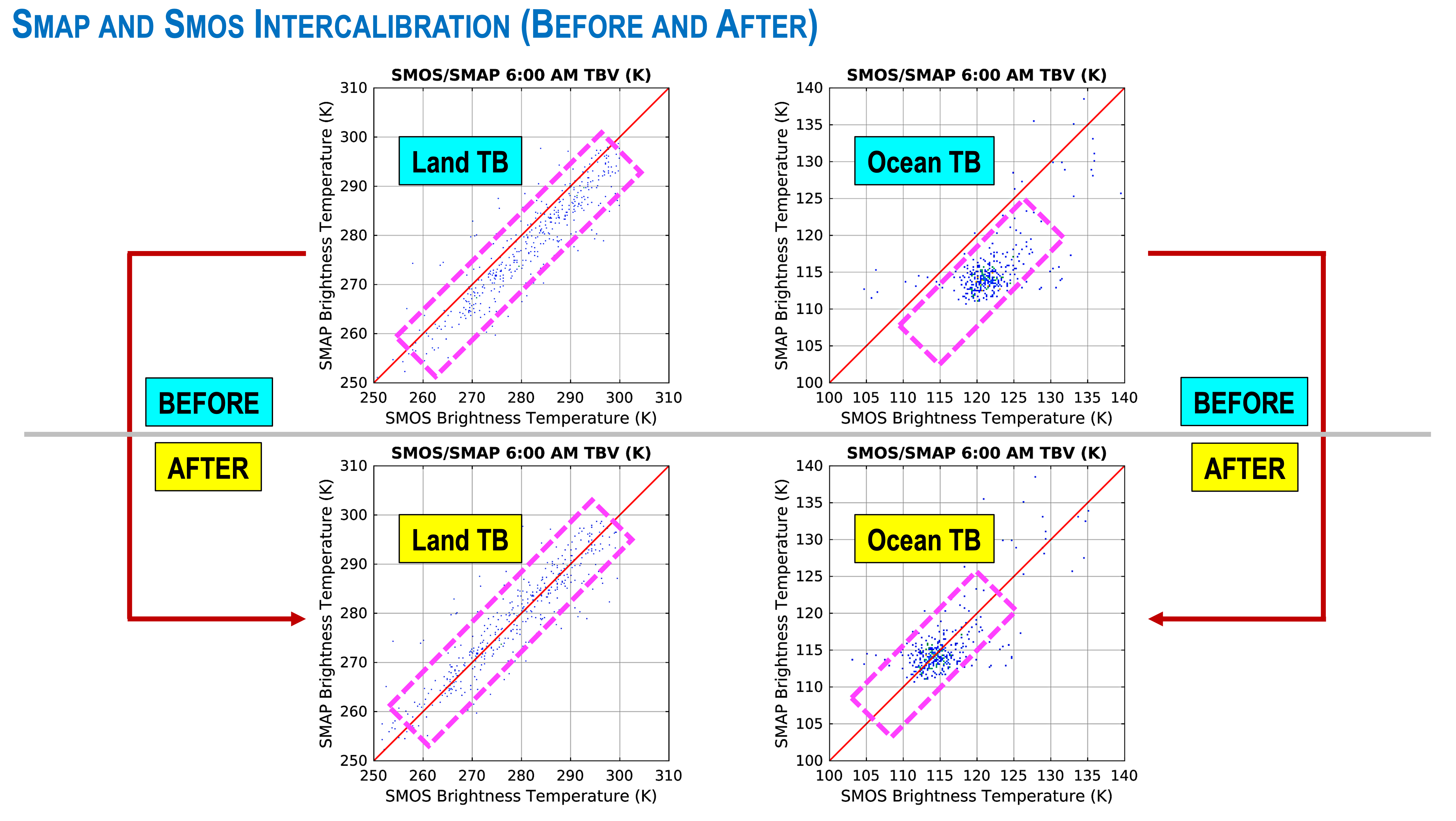
It is important to note also the limitations of this regression approach based on matchup pairs. No matter how stringent these colocation criteria are, they do not eliminate the impacts of the natural uncorrelated radiometric noise (NEΔT) present in both instruments. The regression coefficients determined from these matchup pairs will always be subject to this additional uncertainty.
X-band (10.7 GHz; λ ~ 3 cm)
To achieve consistent calibration among the X-band radiometer observations used in this investigation, we will directly leverage the consistent cross calibration work behind the development of the Global Precipitation Mission (GPM) Level 1C Common Calibrated Brightness Temperature Data Product. This product uses the GPM Microwave Imager (GMI) Level 1B brightness temperature observations as the calibration reference standard for all other radiometer observations within the GPM constellation, including those observations from TMI on NASA TRMM, AMSR-E on NASA Aqua, WindSat on Navy Coriolis, AMSR2 on JAXA GCOM-W, and GMI on NASA GPM. The Algorithm Theoretical Basis Document (ATBD) of this Level 1C product can be found at https://gpm.nasa.gov/resources/documents/gpm-level-1c-algorithm-theoretical-basis-document-atbd. The consistency in calibration among these radiometer observations forms the foundation of the GPM Level 3 Integrated Multi-satellitE Retrievals for GPM (IMERG) precipitation data product. A complete document for all GPM products, including the Level 1C Common Calibrated Brightness Temperature Data Product, can be found here.
Product Grid Projection
The soil moisture estimates produced in this investigation are stored on an Earth-centered, Earth-fixed (ECEF) coordinate system known as the Equal-Area Scalable Earth Grid (EASE-Grid) projection developed by the National Snow and Ice Data Center. There are global, north polar and south polar projection families within the EASE Grid formulation, only the global projection is used in this investigation.
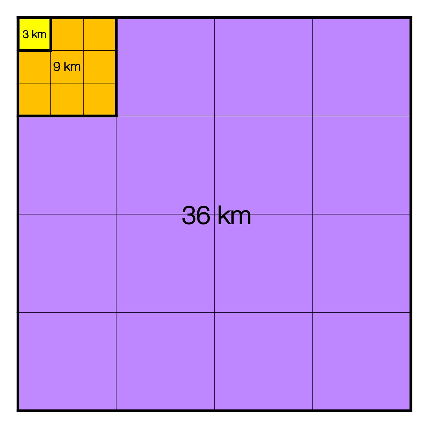
On an EASE Grid projection, data elements are stored in 2-D arrays referenced by row and column indices, making it possible to apply complicated vectorized numerical operations to a large number of data points over any arbitrary shape of region on the Earth surface. Furthermore, data arrays of grid resolutions that are integer multiples of one another are perfectly nested with one another, as shown in the following figure for the case of 3, 9, and 36 km. This simplifies data transition or exchange from one grid resolution to another without complicated interpolation.
For all grid resolutions under this projection, all grid cells have the same nominal area given by the square of their respective grid resolution. This property thus makes it trivial for surface area estimation without causing areal distortion at a function of latitudes. The EASE Grid projection has a decades-long heritage within the cryosphere and terrestrial hydrology communities; it integrates well with free and commercial Geographic Information System (GIS) software.
Product Grid Resolution
The various L- and X-band radiometers all have their own unique viewing geometry, sampling density, footprint size, etc. Some of them (e.g. SMOS) do not have a spinning antenna for data acquisition, others (e.g. AMSR-E and AMSR2) do. Among those that do, some (e.g. SMAP) collect data in both fore- and aft-directions, whereas some (e.g. AMSR-E and AMSR2) do so in only one direction. It is a challenge to settle on a grid posting for storing time-ordered brightness temperature observations by a given radiometer without some quantitative image analyses on the resulting gridded brightness temperature images.
To this end, we used a widely applied perception metric known as the Structural Similarity (SSIM) index to quantify the perceived change in structural information in a brightness temperature image produced at one grid resolution to another. The SSIM formulation was first described in the following publication:
Wang, Z., A. C. Bovik, H. R. Sheikh and E. P. Simoncelli, "Image quality assessment: from error visibility to structural similarity," in IEEE Transactions on Image Processing, vol. 13, no. 4, pp. 600-612, April 2004, doi:10.1109/TIP.2003.819861.
As grid resolution becomes finer and finer, successive brightness temperature images would become more and more similar. This would continue until empty pixels begin to appear when the underlying grid resolution becomes finer than the sampling resolution of the original time-ordered brightness temperature observations. An optimal grid resolution is one where any further increase in grid resolution will no longer result in a substantially different image before empty pixels appear. The following figure series depicts how structural similarity index varies from one grid resolution to another, starting with the index that measures the similarity between the brightness temperature image at a 72 km grid resolution and itself (thus an SSIM value of 1.000).
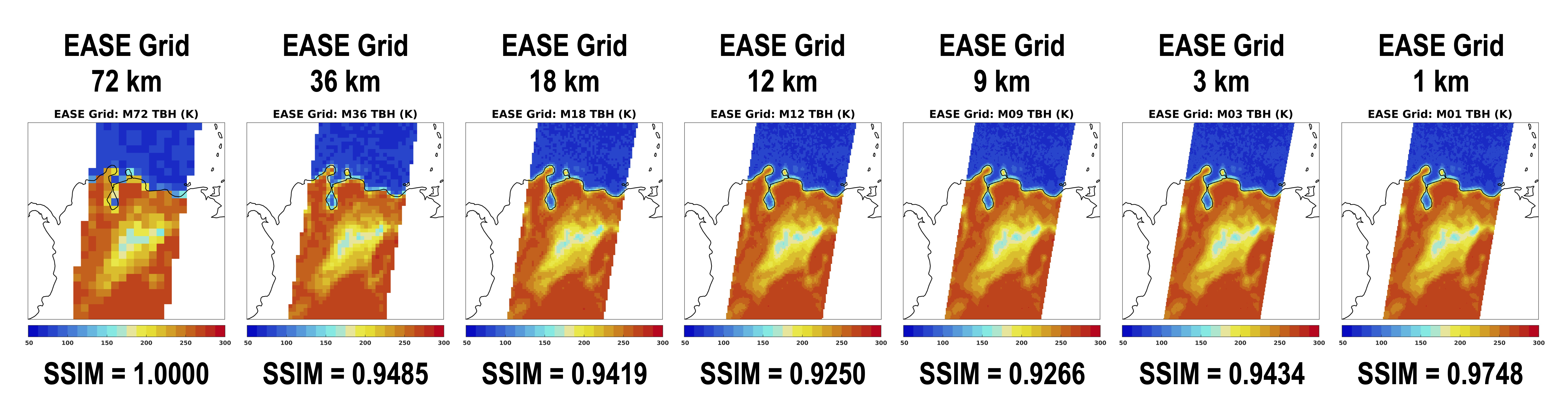
As grid resolution varied from 72 km to 36 km, the SSIM dropped by 5.15% from 1.0000 to 0.9485, implying that the "saturation" of structural information had not arrived yet. From 36 km to 18 km, SSIM continued to drop but to a smaller extent (0.95%) than before; then from 18 km to 12 km, another SSIM drop was observed.
From 12 km to 9 km, however, the first SSIM increase was observed. In other words, the structural information in the two brightness temperature images is essentially the same between these two grid resolutions -- the use of a 9 km EASE Grid projection effectively yielded no new information. This upward trend in SSIM continued from 9 km to 3 km, followed by 3 km to 1 km. It is thus clear that beginning around 9 km, images became more and more similar as grid resolution became finer and finer.
Based on this analysis, one may conclude that soil moisture estimates derived from L-band radiometer observations are most optimally stored on a 9 km EASE Grid projection. A grid resolution finer than 9 km will not capture any new structural information (because there is no more), whereas a grid resolution coarser than 9 km will likely miss residual structural information that is still available in the data. Note that the observed SSIM variability in this particular example did not have anything to do with the ragged swath edges that vary from one image to another. The same conclusion remained after all images were trimmed to share the same ragged swath edges in the M72 image in another separate analysis.