Ancillary Data
Geophysical inversion of soil moisture from passive microwave observations requires external ancillary data. These ancillary data serve to provide correction for geophysical parameters whose radiometric contributions could confound retrieval of soil moisture estimates. Below is a list of ancillary data used for geophysical correction in this investigation.
Coastal and Inland Open Water
Modern radiometers have a finite field-of-view (FOV) on earth surface that varies a few kilometers to tens of kilometers, depending on the antenna size and observation frequencies. When water enters into FOV in a mixed scene of water and land as over coastlines or around large inland open water bodies like lakes or wetlands, the resulting passive microwave observations will contain radiometric contributions by water and land within the FOV. Without proper correction, direct retrieval of soil moisture would likely result in a wet bias. Mitigation of this confounding source to soil moisture estimation requires knowledge of the location and temperature of coastal/inland open water. Location information indicates where water brightness temperature should be taken out; temperature information indicates how much water brightness temperature should be taken out.
There are many high-quality global land/water data products with varying resolution, accuracy and latency; these products are more than adequate in addressing the location need stated above. Comparatively speaking, however, there are not many global inland water temperature data products that address the associated water temperature need. The following article provides a survey of several available inland water temperature data products and explores their utility in the context of passive remote sensing of soil moisture. It was concluded that in order to accommodate the wide variety of spatial and temporal coverage of satellite passive microwave observations, model-based data products at the highest available resolution and temporal frequency with regular operational/reanalysis production schedule is the only viable solution.
Zhang, Runze; Chan, Steven; Bindlish, Rajat; Lakshmi, Venkataraman. 2021. "Evaluation of Global Surface Water Temperature Data Sets for Use in Passive Remote Sensing of Soil Moisture," Remote Sens. 13, no. 10: 1872. https://doi.org/10.3390/rs13101872
Based on these considerations, the ECMWF ERA5-Land 0.1° x 0.1° Hourly (1981-Present) Data Product was identified in the article to be the most optimal dataset that would provide global inland water temperature data through the lake mix-layer temperature data field. This data field is a global data field, meaning that it has nonzero value everywhere over land and ocean. To identify temperature over only coastal and inland water areas, an underlying static lake cover fraction data array from the ECMWF ERA5 0.5° x 0.5° Hourly (1979-Present) Data Product is required by design. This data array specifies the proportion of a grid box covered by inland water bodies (lakes, reservoirs, rivers and coastal waters). Values vary between 0: no inland water, and 1: grid box is fully covered with inland water. In this investigation, a lake cover fraction greater than or equal to 0.50 is used alongside the lake mix-layer temperature data field to assign temperature over inland water areas, and also alongside the sea surface temperature data field to assign temperature over coastal areas. Lake cover fraction less than this threshold over is considered as land whose multilayer soil temperatures will be assigned from the soil_temperature_level_[1-4] from the same ECMWF ERA5-Land 0.1° x 0.1° Hourly (1981-Present) Data Product. A separate static land cover fraction data array delineates where the sea surface temperature and the soil_temperature_level_[1-4] data fields are assigned globally. Both the lake cover fraction and land cover fraction maps are available as standalone data arrays downloadable from the Copernicus Climate Change Service (C3S). These two static cover fractions are illustrated in the following figures:
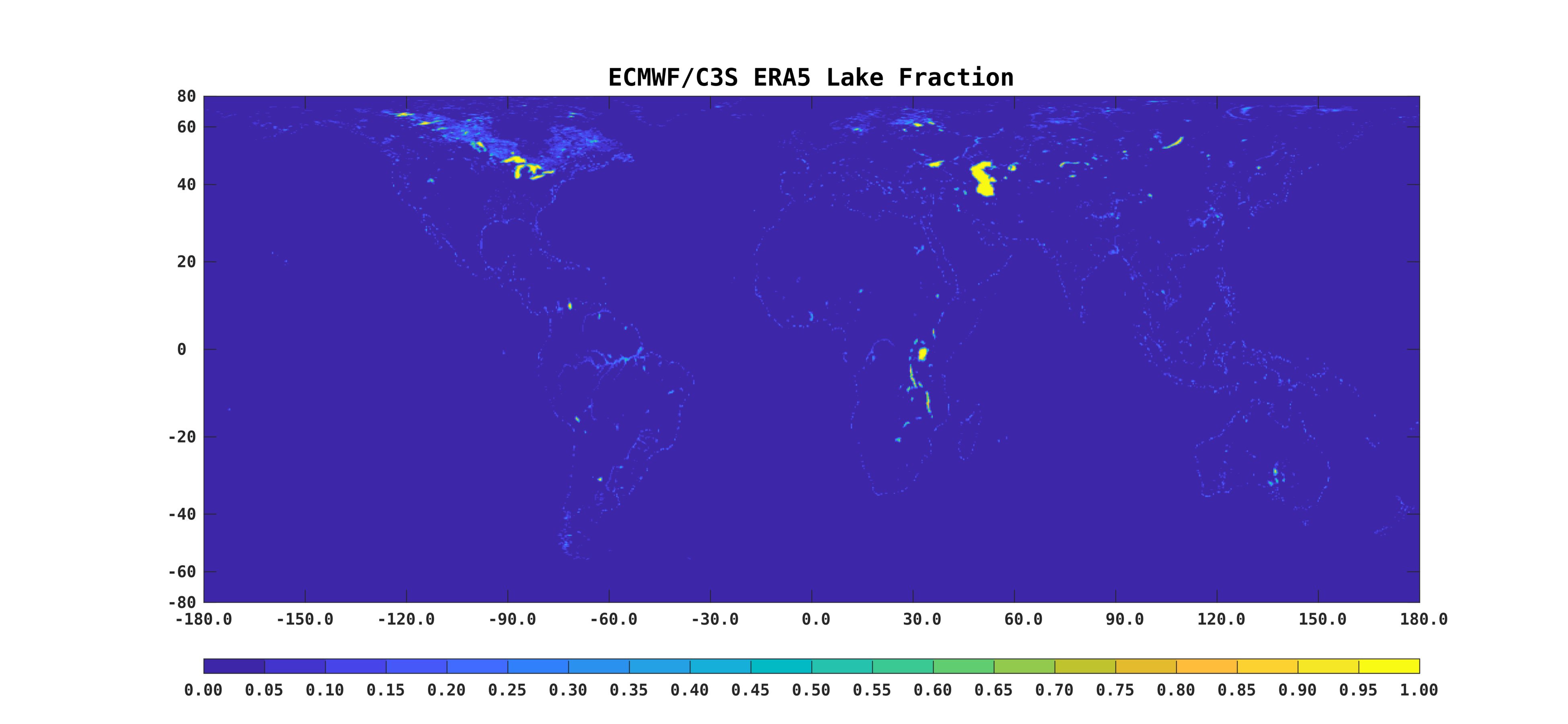
Lake cover fraction
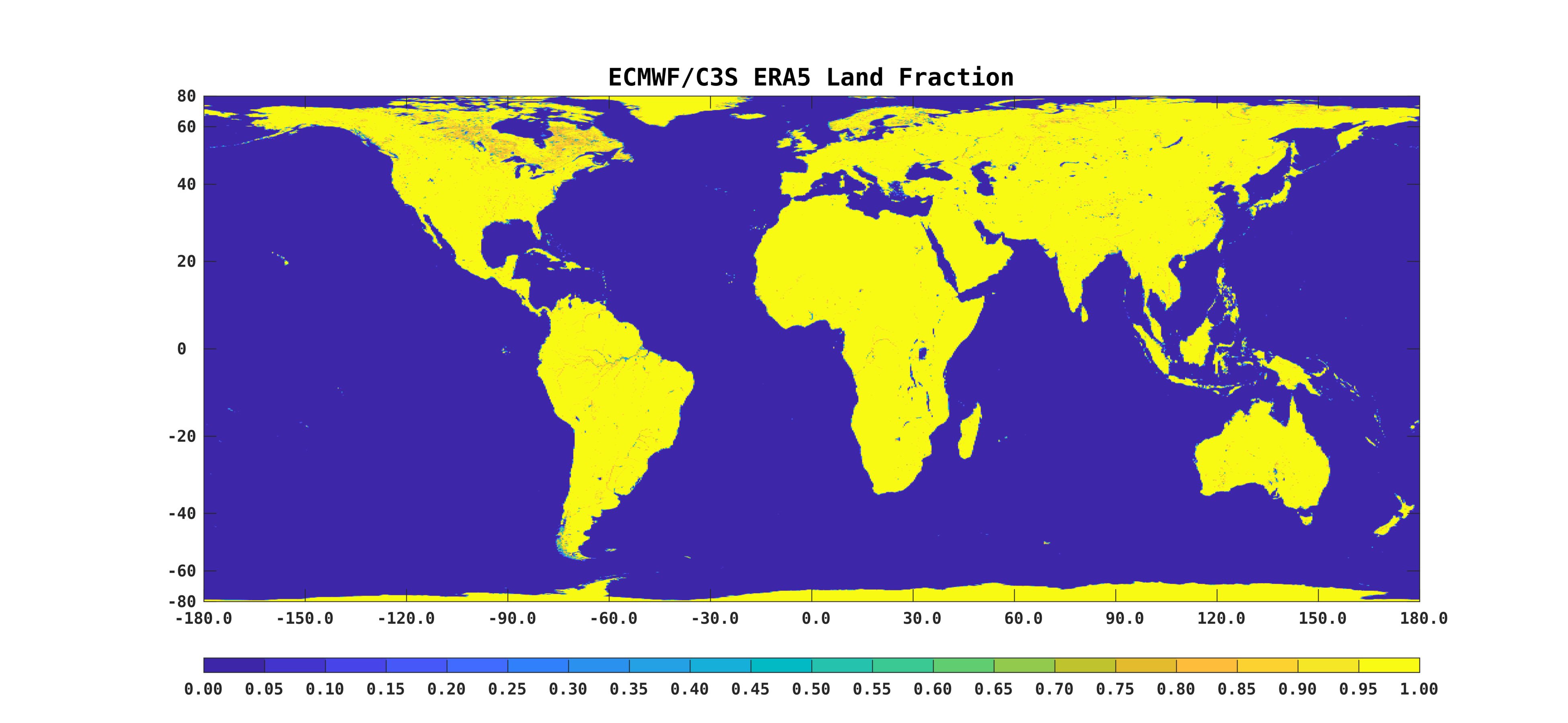
Land cover fraction
Vegetation Index
Emission from vegetation poses another confounding factor that needs to be corrected. For a given brightness temperature measurement at a fixed effective soil temperature, uncorrected emission from vegetation would lead to a soil moisture estimate that is lower than the reality according to the τ-ω inversion model. This misinterpretation would lead to an undesirable dry bias in soil moisture estimates. To properly correct for the impact of vegetation emission, the same correction approach used in SMAP is used in this investigation. In particular, the Version 6 MODIS/Terra Vegetation Indices 16-Day L3 Global 1 km SIN Grid (MOD13A2) data between 2000-2021 were used to produce a long-term Normalized Difference Vegetation Index (NDVI) climatology. This long-term averaging process has both pros and cons. By averaging over a such a long time span, the natural fluctuations between adjacent NDVI measurements can be reduced significantly. Also, missing data due to transient cloud contamination or blockage becomes less of an issue. Although this long-term averaging process can improve the resulting NDVI climatology data quality, it also hinders its capability to capture recent trends of variability. For example, regions that have undergone ongoing greening (gaining vegetation) or browning (losing vegetation) recently would not be represented accurately by such a long-term climatology. After extensive studies, however, we concluded that a long-term NDVI climatology leads to better soil moisture retrieval performance than, for example, what a moving 5- or 10-year averaged NDVI climatology offers.
This NDVI climatology is then interpolated spatially on a 3-km EASE Grid and then also temporally at a daily interval for a 366-day span in order to account for leap years. To generate the proper amount of vegetation emission correction, the same SMAP approached described in the following document is used. In essence, NDVI at a given location and time is combined with a static landcover-based lookup table of coefficients described in the following document to produce an empirical estimate of the vegetation opacity (τ) (a.k.a. vegetation optical depth). The resulting vegetation opacity is then used as an input to the τ-ω inversion model to solve for an estimate of soil moisture. The exact procedures of VWC reconstruction from NDVI is described in the following documents:
Chan, Steven, et al. 2013. "SMAP Ancillary Data Report: Vegetation Water Content," Jet Propulsion Laboratory, California Institute of Technology, JPL D-53061. URL: https://smap.jpl.nasa.gov/system/internal_resources/details/original/289_047_veg_water.pdf. Accessed: May 31, 2022.
O'Neill, Peggy, et al. 2020. "SMAP Algorithm Theoretical Basis Document: Level 2 and 3 Soil Moisture (Passive) Products," Jet Propulsion Laboratory, California Institute of Technology, JPL D-66480. URL: https://smap.jpl.nasa.gov/system/internal_resources/details/original/484_L2_SM_P_ATBD_rev_F_final_Aug2020.pdf. Accessed: May 31, 2022.
An up-to-date inventory of this database can be found on the LP DAAC server.
Effective Soil Temperature
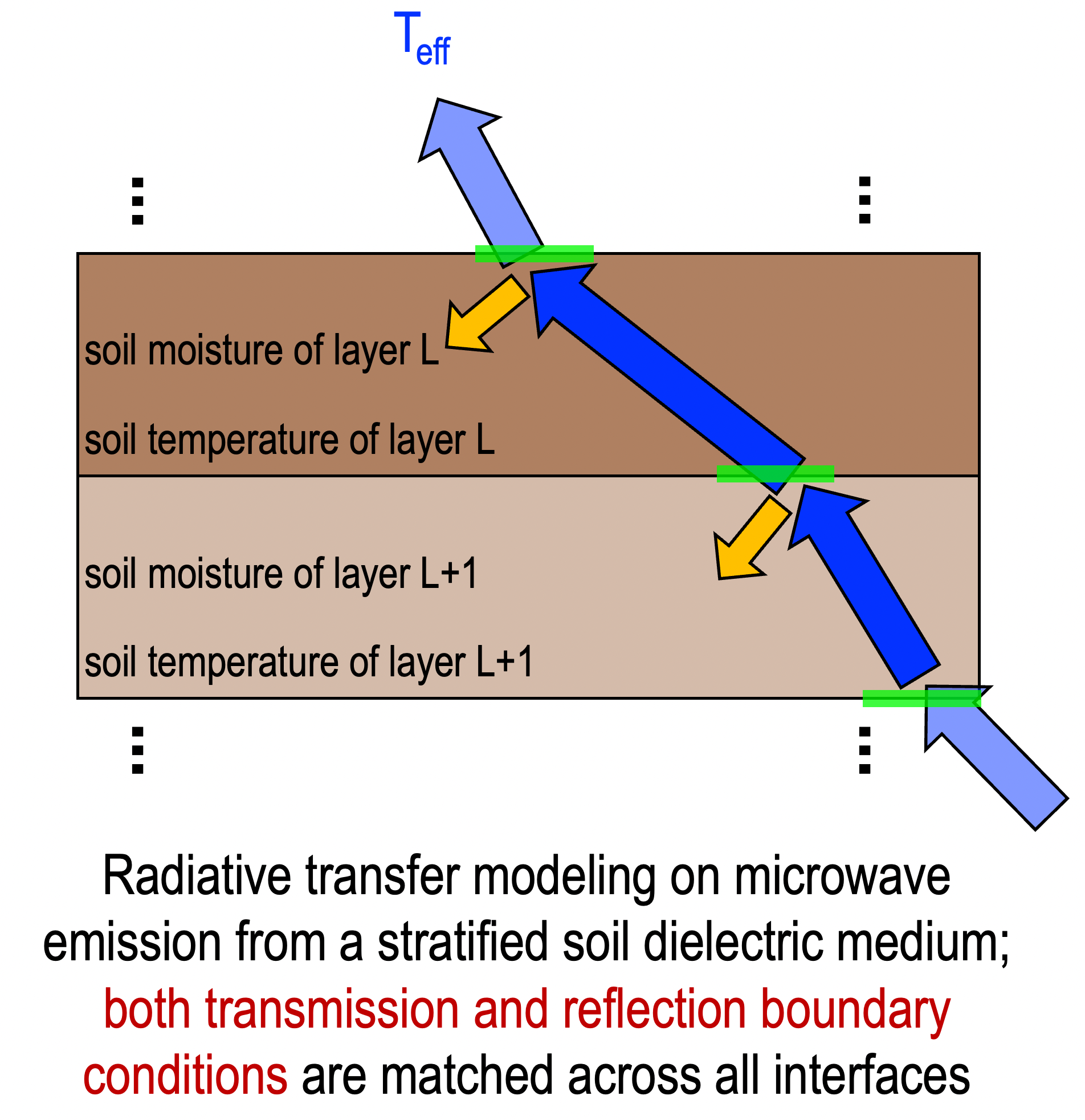
In classical radiative transfer theory, the brightness temperature from a soil medium can be modeled as the product between soil emissivity and effective soil temperature. In the context of soil moisture retrieval from TB observations, Teff is a key parameter that provides temperature correction -- too high Teff would lead to
TB = e Teff
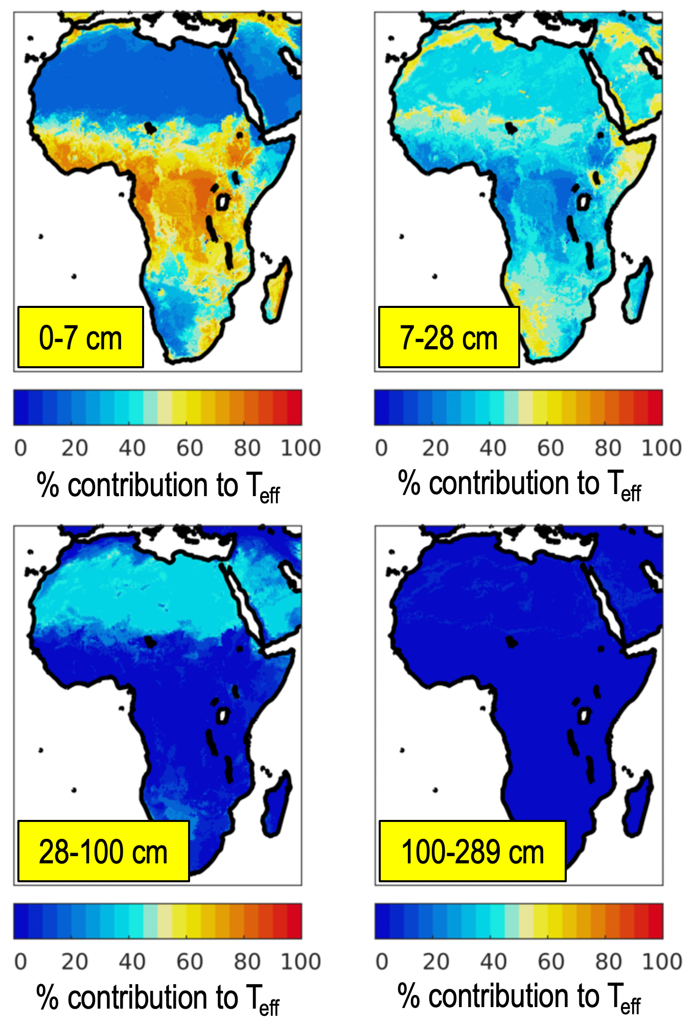
For a soil medium modeled as a stratified medium consisting of multiple layers of lossy dielectric materials characterized by unique complex dielectric constants, soil emissivity (e) is primarily a function of soil moisture of the first soil layer, followed by its dependence on the observed frequency, polarization, and incidence angle. The effective soil temperature (Teff), on the other hand, is a function of soil moisture and soil temperature from all layers, in addition to its dependence on the observed frequency, polarization, and incidence angle. To compute Teff analytically, we use the same ECMWF ERA5-Land 0.1° x 0.1° Hourly (1981-Present) Data Product mentioned in the "Coastal and Inland Open Water" section above to extract global hourly snapshots of volumetric_soil_water_layer_[1-4] and soil_temperature_level_[1-4] in our calculations. In ERA5, the soil depths associated with these two layered parameters go from 0-7 cm, 7-28 cm, 28-100 cm, and 100-289 cm. Through meticulous algebraic efforts later verified with the help of commercial symbolic math software, we obtained the full analytical radiative transfer solution to the microwave emission from a 4-layer soil medium as a function of frequency, polarization, incidence angle, and layer properties. This solution has been coded in a vector manner so that global Teff calculations can be conducted in a fraction of time. Note that we also obtained similar analytical solutions for a 5- and 6-layer soil medium, but the solutions are too long to be included here. In what follows, β will be used to denote either the horizontal (h) or vertical (v) polarization under consideration.
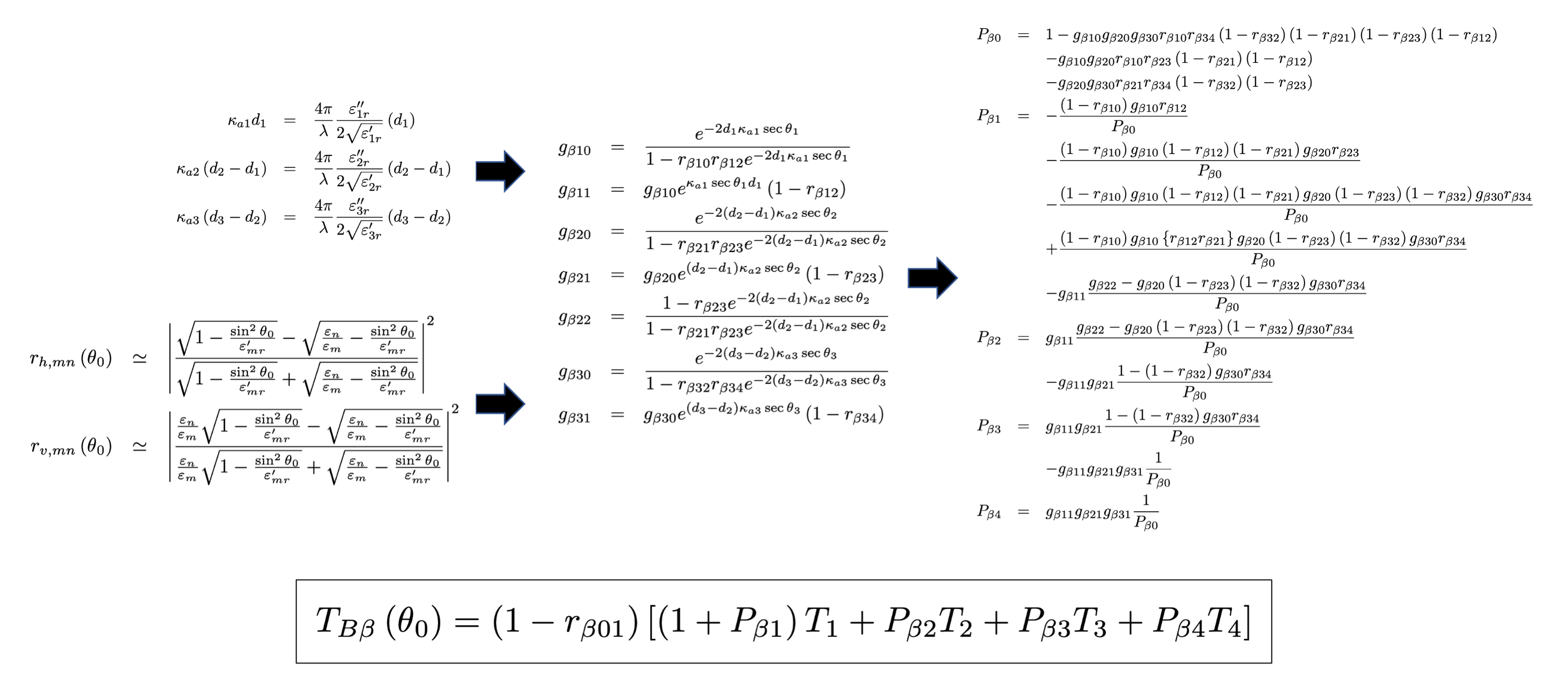
A few notes on this analytical solution of TB:
- This follows the form of TB = e Teff, with the first term representing the soil emissivity (e) and the second term the effective soil temperature.
- Because both e and Teff are functions of frequency, polarization, and incidence angle, this analytical solution of TB can be used to model horizontally or vertically polarized brightness temperature observations acquired by radiometers observing at different incidence angles and different frequencies.
- The same Teff term can be used to compute effective soil temperature at different times during the day throughout the entire diurnal cycle, driven by the underlying hourly volumetric_soil_water_layer_[1-4] and soil_temperature_level_[1-4] data in the ECMWF ERA5-Land 0.1° x 0.1° Hourly (1981-Present) Data Product. Although Teff has a theoretical dependence on polarization and incidence angle, our calculations have shown that this dependence is negligible.
- A soil dielectric model is needed to provide the real and imaginary part of soil dielectric constant for each layers. In this investigation, we will use the same soil dielectric model used in SMAP: Mironov, V, et al. 2009. Physically and Mineralogically Based Spectroscopic Dielectric Model for Moist Soils, IEEE Transactions on Geoscience and Remote Sensing, 47(7), pp. 2059 - 2070, DOI:10.1109/TGRS.2008.2011631
- For a stratified medium having more than four layers, it is more tractable to formulate this radiative transfer description in matrix form and solve for the numerical solution directly. This matrix-based procedure is described in Tsang, et al. 2000, Scattering of Electromagnetic Waves: Theories and Applications, Chapter, 5, Vol. 1, John Wiley & Sons, Inc. Both coherent and incoherent formulations were implemented in this investigation. Note that this matrix-based solution will lead to the direct modeling of TB; Teff can still be computed by TB / e; however, its dependence on soil temperature partition among individual soil layers will require symbolic math software for an analytical solution.
- This formulation is an extension of works described previously in Lv, et al. 2014, 2016, and 2019, in that both transmission and reflection of specific intensity across layers are explicitly modeled here. This modeling of reflection is an important consideration not accounted for in previous works because vertical gradient of soil moisture will lead to mismatch in soil dielectric constant, causing intensity reflections between adjacent soil layers.
- Teff can be seen as a linear superposition of soil_temperature_level_[1-4], with individual coefficients depending on soil moisture and soil temperature from all layers, in addition to its dependence on the observed frequency, polarization, and incidence angle. Below is a sample run of Teff based on the vast spatial diversity of soil moisture distribution over the African continent. It is clear that Teff is a strong function of soil depths especially where soil moisture is low. If only the soil temperature from the first is used to estimate Teff over these regions, any potential bias in Teff estimation will lead bias in soil moisture estimation. It is also evident from the following figures that Teff is also strongly dependent on soil moisture, meaning that soil moisture estimate should be retrieved from both the surface emissivity (e) term and the effective soil temperature (Teff) term in TB = e Teff, rather than just from the surface emissivity (e) term as in SMAP.
Soil Attributes
Soil attributes are another essential database in this investigation. Following the same relationship TB = e Teff above, this database primarily plays two roles in this investigation. First, it provides the conversion from soil moisture in the top soil layer to complex dielectric constant (ε' + jε''), where ε' and ε'' represent respectively the real and imaginary part of soil dielectric constant. Knowledge of ε' and ε'' can be used to estimate the Fresnel reflectivity and thus the surface emissivity. Second, the same conversion also specifies the complex dielectric constants based on the values of volumetric_soil_water_layer_[1-4] data in the ECMWF ERA5-Land 0.1° x 0.1° Hourly (1981-Present) Data Product. These complex dielectric constants are then used in the analytical formulation of Teff described above.
The OpenLandMap soil attribute database will be used in this investigation. This collection was chosen because it represents a large compilation of soil data published by various national and international soil data providers:
- USDA National Cooperative Soil Characterization Database,
- Africa Soil Profiles Database,
- LUCAS Soil database,
- Repositório Brasileiro Livre para Dados Abertos do Solo (FEBR),
- Sistema de Información de Suelos de Latinoamérica y el Caribe (SISLAC),
- The Northern Circumpolar Soil Carbon Database (NCSCD),
- Dokuchaev Soil Science Institute / Ministry of Agriculture of Russia (soil profiles for Russia),
- WHRC global mangrove soil carbon dataset,
- Local data sets such as Silva et al. (2019),
The published data were then used in a machine learning framework to create a global database of soil attributes at a 250-meter resolution at six soil depths (0, 10, 30, 60, 100 and 200 cm). The exact specifications can be found here. The following soil attribute parameters were processed on 3- and 9-km EASE Grid 2.0 projections for this investigation.
- Sand fraction: Sand content in % (kg / kg) at 6 standard depths (0, 10, 30, 60, 100 and 200 cm) at 250 m resolution (Download: https://zenodo.org/record/2525662)
- Clay fraction: Clay content in % (kg / kg) at 6 standard depths (0, 10, 30, 60, 100 and 200 cm) at 250 m resolution (Download: https://zenodo.org/record/2525663)
- Silt content: Silt content in % (kg / kg) at 6 standard depths (0, 10, 30, 60, 100 and 200 cm) at 250 m resolution (Download: https://zenodo.org/record/2525676)
- Soil organic carbon content: Soil organic carbon content in x 5 g / kg at 6 standard depths (0, 10, 30, 60, 100 and 200 cm) at 250 m resolution (Download: https://zenodo.org/record/2525553)
- Bulk density: Soil bulk density (fine earth) 10 x kg / m-cubic at 6 standard depths (0, 10, 30, 60, 100 and 200 cm) at 250 m resolution (Download: https://zenodo.org/record/2525665)
- Soil water content at 33 kPa (under extreme wet soil condition): Soil water content (volumetric %) for 33 kPa suction predicted at 6 standard depths (0, 10, 30, 60, 100 and 200 cm) at 250 m resolution (Download: https://zenodo.org/record/2784001)
- Soil water content at 1500 kPa (under extreme dry soil condition): Soil water content (volumetric %) for 1500 kPa suction predicted at 6 standard depths (0, 10, 30, 60, 100 and 200 cm) at 250 m resolution (Download: https://zenodo.org/record/2784001)
Note that these standard depths are different from those specified in the ECMWF ERA5-Land 0.1° x 0.1° Hourly (1981-Present) Data Product, linear interpolation on these soil attributes was conducted to remap these depths from 0-10 cm, 10-30 cm, 30-60 cm, 60-100 cm, and 100-200 cm to 0-7 cm, 7-28 cm, 28-100 cm, and 100-289 cm.
Land Cover Classification
The same MODIS/Terra+Aqua Land Cover Type Yearly L3 Global 500 m SIN Grid (MCD12Q1) Data Product used in SMAPis also used in this investigation and for the same purposes. This database defines a lookup table that adjusts the behavior of geophysical inversion of soil moisture as well as the amount of vegetation correction needed in the inversion process. This lookup table and the vegetation correction procedure were described in the SMAP Algorithm Theoretical Basis Document as follows:
O'Neill, Peggy, et al. 2020. "SMAP Algorithm Theoretical Basis Document: Level 2 and 3 Soil Moisture (Passive) Products," Jet Propulsion Laboratory, California Institute of Technology, JPL D-66480. URL: https://smap.jpl.nasa.gov/system/internal_resources/details/original/484_L2_SM_P_ATBD_rev_F_final_Aug2020.pdf. Accessed: May 31, 2022.
At present, the (MCD12Q1) data product is current up to 2020. A more up-to-date inventory of this database can be found on the LP DAAC server.
Others
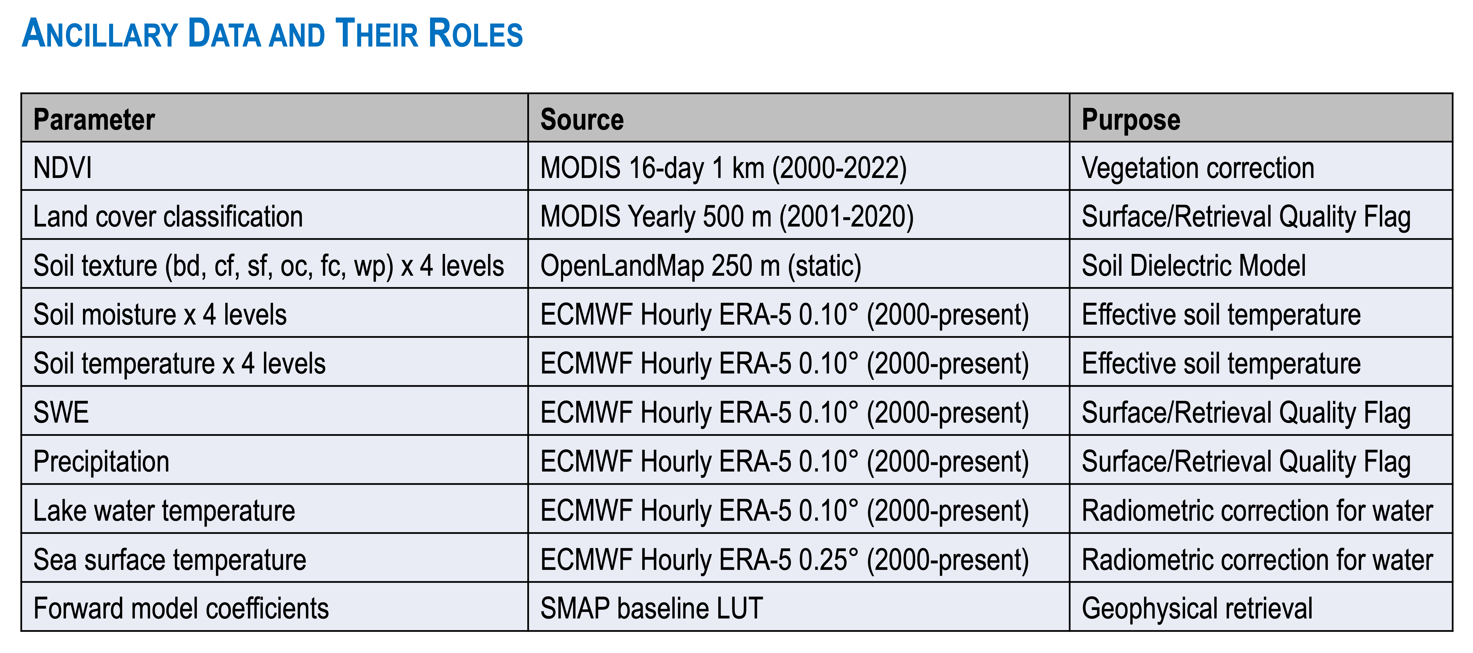
There are other ancillary data not listed above but were used in this investigation. The specifications of these ancillary data, along with those already mentioned above, are summarized in the following table: